Harmonic response visualization used to identify resonance-driven amplification and critical deformation behavior.
Executive summary
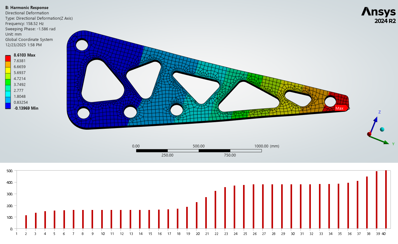
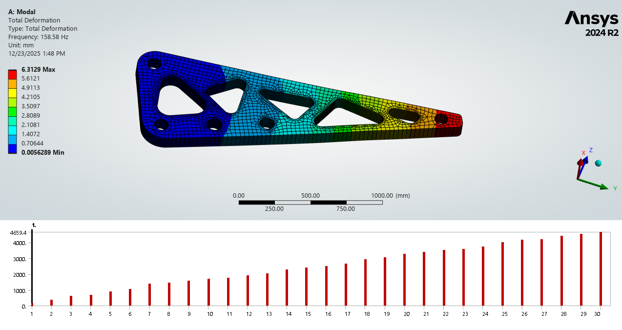
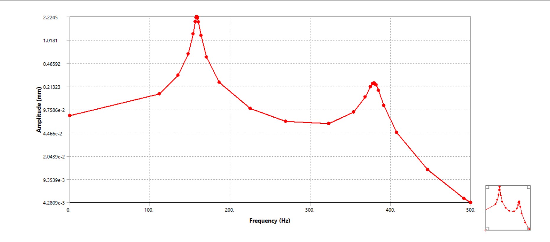
- Dominant resonance: ~158.5 Hz (primary amplification region)
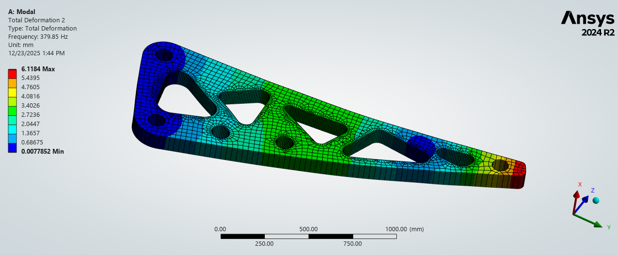
- Secondary resonance: ~380 Hz
- Peak deformation (at resonance): ~8.6 mm (directional Z)
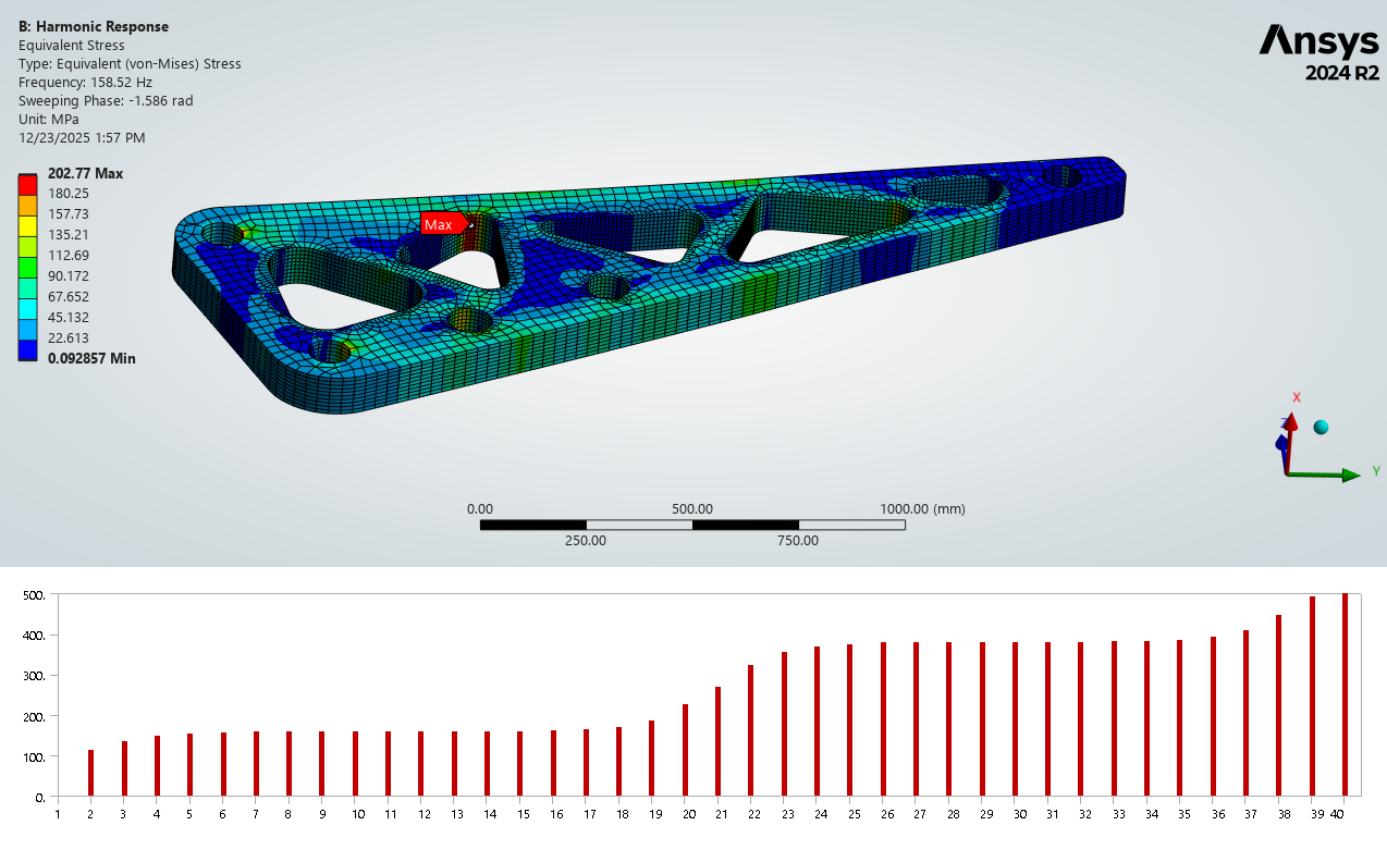
- Peak alternating stress: ~202 MPa (equivalent von Mises)
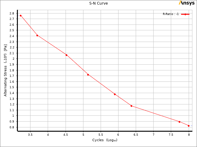
Fatigue result (S–N)
- Minimum predicted life: ~253 s at the critical hotspot
- Method: Stress–Life (S–N), fully reversed (R = −1)
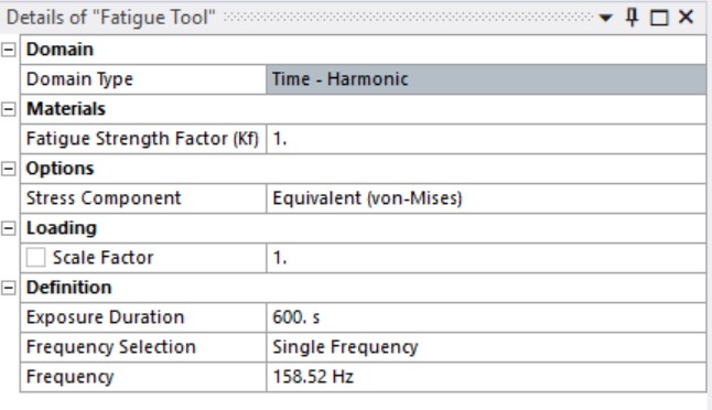
- Domain: Time – Harmonic
- Evaluation: single-frequency assessment at 158.52 Hz
Overview
Harmonic loading can produce response levels far above static expectations when the excitation aligns with a structure’s natural frequencies. In such cases, resonance-driven amplification elevates deformation and stress, often creating localized hotspots where fatigue cracks initiate. This workflow combines modal analysis, harmonic response, and stress–life fatigue to support design decisions early—before physical testing.
Why this matters: The same 10 kN load can be “safe” away from resonance but damaging near resonance. Identifying frequency-sensitive amplification regions is essential for robust durability design.
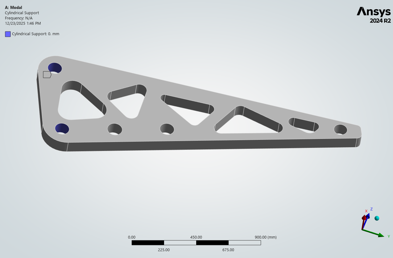
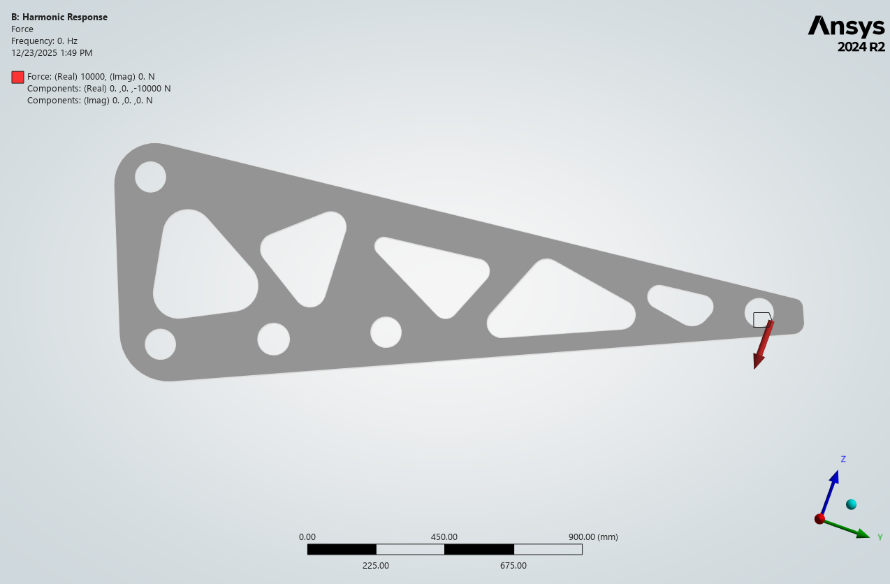
1) Model setup
The bracket is constrained at mounting locations using cylindrical supports. A 10,000 N harmonic force is applied at the free-end hole to represent periodic excitation during operation.
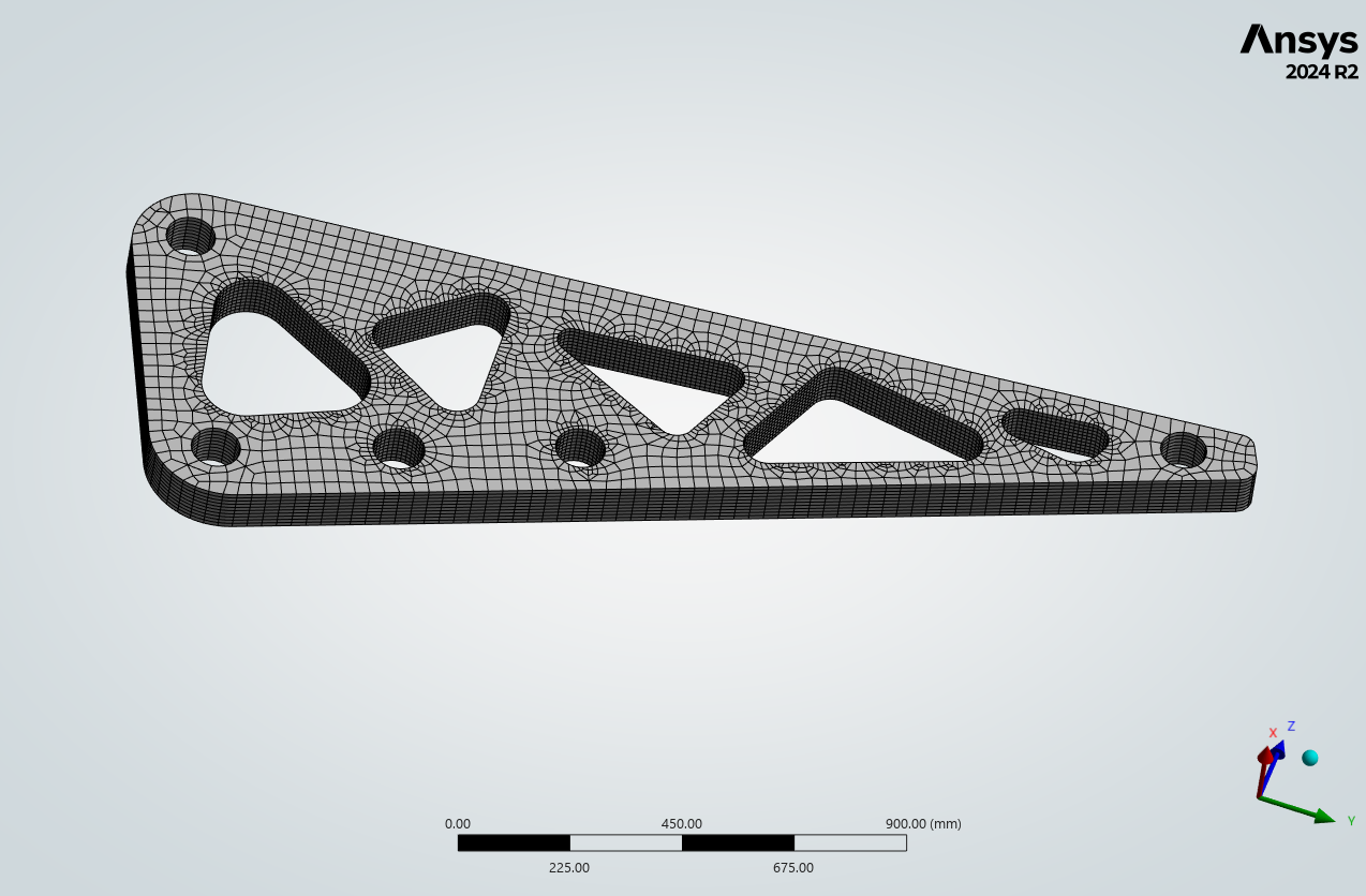
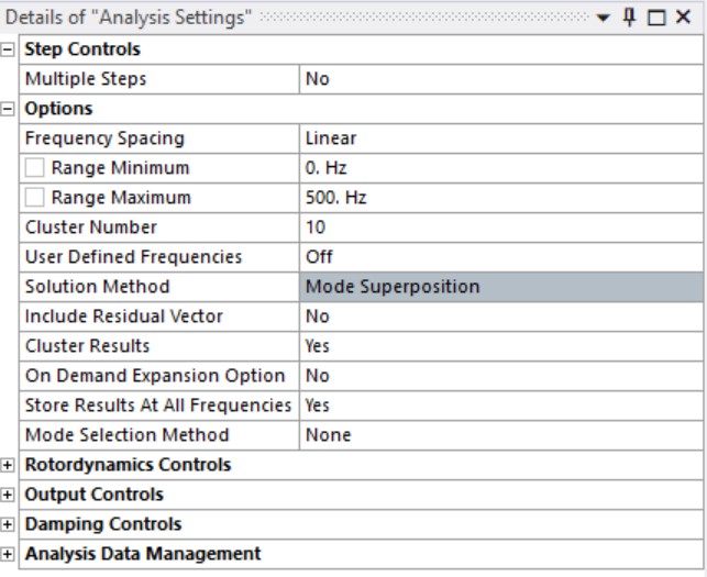
2) Mesh and harmonic analysis settings
A 3D solid mesh is used with refinement near geometric discontinuities (holes and cutouts) to resolve stress gradients. The harmonic response is solved using mode superposition over 0–500 Hz with linear spacing.
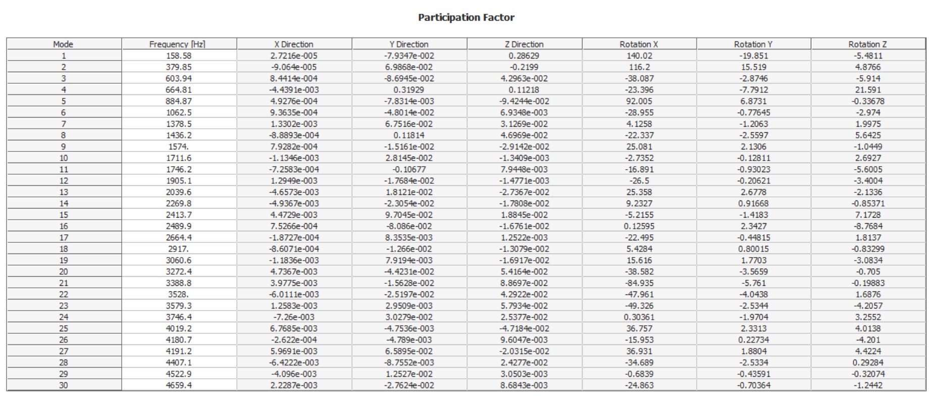
3) Modal results and resonance drivers
Modal analysis identifies natural frequencies and mode shapes that drive harmonic amplification. The frequency response indicates a dominant amplification region near ~158.5 Hz and a secondary region near ~380 Hz.
4) Phase response
The phase plot shows a rapid transition across resonance (approximately π radians), which is a classic signature of a resonant system. This confirms the peak near ~158.5 Hz is resonance-driven rather than a static-like trend.
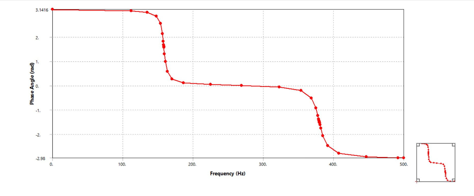
Phase angle vs. frequency — sharp phase change across resonance.
5) Harmonic stress and deformation at the critical frequency
At the dominant resonance (~158.5 Hz), dynamic amplification drives peak deformation and elevated alternating stress. Stress concentrations are localized near holes/cutouts—typical initiation sites for fatigue damage.
6) Fatigue setup
Fatigue life is computed using the Stress–Life (S–N) method. The Fatigue Tool is configured in the Time – Harmonic domain using equivalent (von Mises) stress, evaluated at a single frequency (158.52 Hz) with an exposure duration of 600 s.
7) Fatigue life result
The fatigue life contour highlights the most critical hotspot under resonance conditions. The minimum predicted life is approximately 253 seconds, while non-critical regions show substantially longer life within the plotted range.
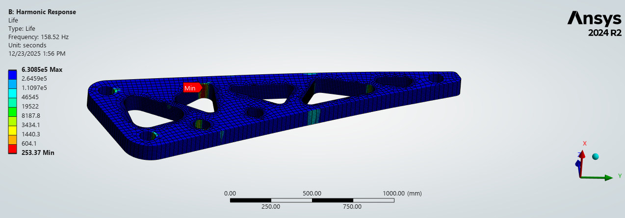
Fatigue life contour at the critical frequency (~158.5 Hz).
Design recommendations
Reduce resonance risk
- Avoid excitation bands: if possible, shift operating conditions away from ~158.5 Hz and ~380 Hz.
- Shift natural frequencies: increase stiffness (ribs/local thickening) or modify geometry to move the modes.
- Add damping/isolation: damping treatments or compliant mounts can reduce amplification near resonance.
Reduce fatigue hotspot severity
- Lower stress concentration: add fillets/smoother transitions near cutouts and holes.
- Local reinforcement: increase section thickness near hotspots if packaging allows.
- Verify fatigue inputs: validate S–N data and mean-stress/damping assumptions for final sign-off.
Need vibration and fatigue support?
We help teams identify resonance risks, quantify dynamic stress, and improve durability with simulation-backed design guidance. Contact us at info@tetraelements.com .
Note: Results shown are from simulation of the presented configuration and analysis settings. Final hardware performance can vary with material properties, damping, boundary conditions, manufacturing tolerances, and real-world excitation profiles.